Deep Learning for Sound-Based Music Recommendation
The status quo in the music recommendation industry is a technique called collaborate filtering. The idea behind collaborative filtering is if person A has indicated that he/she likes the songs “Back In Black” by AC/DC and “Dream On” by Aerosmith, and person B has indicated that he/she likes “Back In Black”, then person B might also like “Dream On”. So the recommendation to person B is “Dream On”, based on the preferences of person A, who shares other common interests. Collaborative filtering relies on data about the preferences of many people. There is a small but growing area of research concerning the recommendation of music based on the music’s sound, rather than metadata like personal preferences. I would argue that this is the way music recommendation should be approached. Imagine the following scenario: you just had an excellent glass of wine at a restaurant, and your waiter comes around to ask you if you’d like another glass. A safe bet would be to ask for another glass of that excellent wine, but being an adventurous person, you would like to try something different, but still good. You ask your waiter to recommend a similar wine. Your waiter could recommend a wine that another patron enjoyed, but a more likely response would be a wine that tastes similar to the wine you just had. This example illustrates that the most important aspect of wine similarity is taste; the way wine affects your senses. Anything else is just “wine metadata”. Why should music be any different? In this article, I will introduce a semi-supervised deep learning model that learns latent features about songs, in order to group similar songs based on sound. The model is able to distinguish songs by musical style and male or female vocalist, and it seems to recognize timbre and instrumentation to some degree. All of my code can be found on GitHub: https://github.com/nlinc1905/Convolutional-Autoencoder-Music-Similarity.
For this experiment, I compiled a dataset of 28 songs. I picked songs from different genres like classical and pop, but also songs that were covered by multiple artists, like Taylor Swift’s and Ryan Adams’ “Bad Blood”. My hypothesis was that songs in different genres would be more different from one another than songs by the same artist or same genre, but songs covered by different artists would be more similar to one another than other songs by those artists. I also included the song “Shakermaker”, by Oasis, and the song “I’d Like to Teach the World to Sing”, by The New Seekers, because Oasis was successfully sued for the melody of their song being too similar to the song by The New Seekers. Listening to the two of them, there are some clear similarities. I wanted to see if those could be captured by a deep learning model.
Before I could analyze the audio files, I had to convert them to a format that could be useful. MP3 format is a stereo, meaning it is comprised of 2 channels of data, typically for left and right speakers. If I were to try to calculate features on that data, there would be 2 possible values for each unit of time. So in order to reduce the data to 1 value per unit time, I converted the files to wav format and picked 1 channel to convert the audio to mono, using the FFPMEG converter (https://FFMPEG.org). I decided to pick one channel rather than mathematically combining the two, but stereo to mono conversion is not lossless: some information will be lost because it only existed in the channel that was removed. To put the loss of information into perspective, think about going to the orchestra. If the violins are positioned to the left of the conductor, and you cover your left ear, you’ll still hear the violins, but you will be hearing more of the echo than the actual signal. Later on, I will list ways that the model can be improved, so keep this point in the back of your mind until then.
Features First Approach
The obvious approach to grouping similar songs would be to apply clustering or some other traditional machine learning technique to features of the music. I used the Python library Librosa to calculate the following audio features:
- Sample Frequency – The number of samples per second, in Hz. MP3 and CD quality music is usually sampled at 44,100 Hz. Since the MP3 files were converted to mono (1 channel) from stereo, the sample frequency was 22,050 Hz for every song.
- Channels – Since the MP3 files were converted to mono, they all had 1 channel.
- Sample points – In order to convert a continuous signal to discrete packets that a computer can understand, sound is sampled. The number of sample points is the number of points along the signal that are taken and compiled into an audio file.
- Audio length (seconds) – The song length in seconds.
- Tempo (beats per minute) – The average number of beats per minute, as estimated by an algorithm in Librosa.
- Average difference between beat times – Librosa estimates the locations of beats in the song to generate tempo. The average difference between estimated beat times gives an idea about changes in tempo throughout the song, when compared to the average tempo.
- Standard deviation in the difference between beat times – Measures standardized variation in the differences between beat times to give an idea about tempo changes throughout the song.
- Roll-off frequency – The maximum frequency in the song, or the frequency at which the audio signal is capped.
- Average zero-crossing rate – The average number of sign changes (positive to negative) along a signal. The zero-crossing rate is commonly used in speech recognition tasks, as voiced segments of audio typically have lower zero-crossing rates.
- Zero-crossing rate range – The range of zero-crossing rates throughout the song.
- Average Mel frequency – The average Mel-scaled frequency.
- Standard deviation in Mel frequency – The standard deviation in Mel-scaled frequencies.
- Average onset strength – Onset strength looks at energy rises across the frequency spectrum to detect the beginning of a note.
- Standard deviation in onset strength – The standardized variation in onset strength throughout the song.
- Tonic – The frequency or pitch upon which all others are referenced. It forms the basis for a key signature.
- Key – The group of frequencies or pitches, including sharps and flats that the song is based on.
- Standardized distance from the average frequency to the tonic – The z-score of the distance from the average frequency to the tonic. This measures the frequency spread of the music.
These features are far from perfect, as I discarded a lot of information by taking the average of many of them, and they’re absolutely not a complete list of possible features that could be calculated, but they are a good starting point. After calculating these features, I used a dimension reduction technique called t-distributed stochastic neighbor embedding (t-SNE) to reduce the dimensions down to 2 and plot the results. Even after tuning the hyperparameters for the t-SNE algorithm, the results did not look good. There were no apparent differences between songs, as everything was plotted in 1 big clump. Songs that were not at all similar sounding were plotted close together. Clearly a different approach was needed.
Deep Learning Approach
The challenge to using deep learning on this data was figuring out how to apply it to an audio signal. I couldn’t simply feed a wav file into a neural network. One idea that has gained some ground in audio analysis using deep learning is to treat the audio data as an image, which then enables the use of tried and true methods for image processing. Audio can be converted to an image by producing a Mel frequency spectrogram, like the one below.
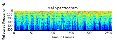
This image shows the frequencies present at any given unit of time in the audio. It does not capture phase information though, so there is some information loss in this approach. Without phase information, it is not possible to reproduce the audio, even with the spectrogram.
Convolutional neural networks are the go-to structures for analyzing image data. They excel at learning spatial structure. I decided to stack convolutional layers in a type of neural network called an autoencoder. Autoencoders are made up of an encoder and a decoder. They perform operations similar to dimension reduction in that they squeeze the input data down to a smaller space in the encoding part, and then decode the encoded image by expanding it back out to the original dimensions in the decoder part. The end result is a reconstruction of the original image. What makes autoencoders useful is that they don’t simply reproduce a given input; they learn latent features about that input. Think of it this way: when you learned to write the alphabet, you were given a picture of what the letter A looked like. Your brain analyzed that picture and instructed your hand how to move to reproduce that letter on paper. The feedback to your brain would be the image that you drew. After repeated attempts to draw the letter A, you finally learned how to do it very accurately. Your brain had learned latent features about the letter A. Autoencoders mimic that process.
The structure of the convolutional autoencoder that I built, using the Python library Keras, looked like this:
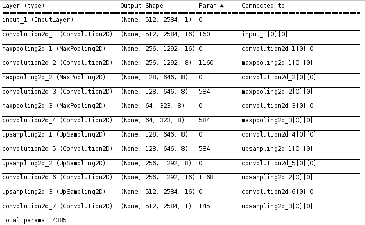
I trained the network using an adaptive learning rate that decreases after each training epoch, with the decay set to learning rate / number of epochs. I used binary cross-entropy loss to evaluate the model at each step, and defined a custom callback function to stop training the autoencoder at 50 epochs or when the validation loss dipped below 0.1, whichever came first. I chose 0.1 after trial and error, as I found that continuing to train beyond that caused the algorithm to overshoot the minimum of the cost function and never recover. None of the autoencoders made it to epoch 50.
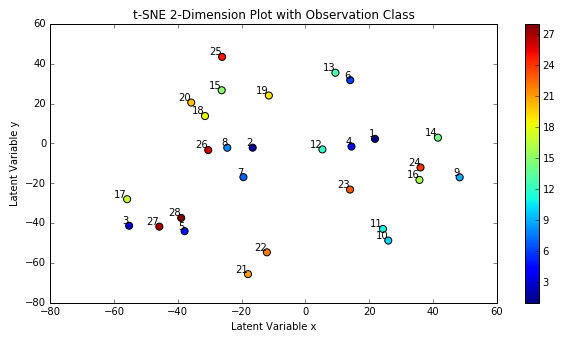
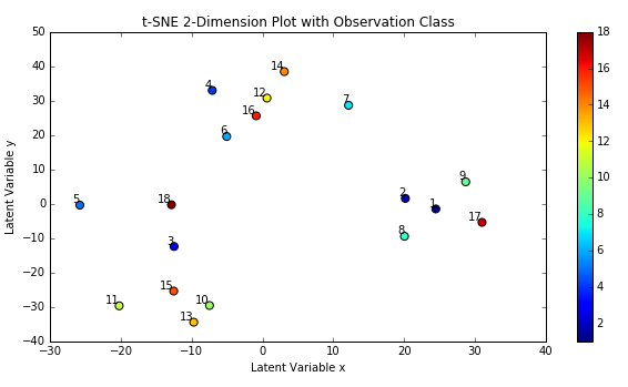
On the first pass, I trained one autoencoder per audio file. I retrieved the encoded Mel spectrogram images, reshaped them into single row vectors and stacked them into a matrix, and then used t-SNE again to reduce the dimensions to 2 so they could be plotted. After trial and error, I found that the optimal parameters for the t-SNE algorithm for this dataset was perplexity of 2 and a learning rate of 100. The plot below shows the results.
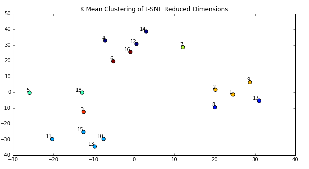
When reading this plot, it’s important to remember that distances between points in a t-SNE plot can be deceiving and not necessarily representative of the differences between points or clusters. To better show clusters, I applied the k-means algorithm to the t-SNE dimensions, which produced the plot below. I used k=8 because looking at the t-SNE plot above seemed to imply there might be 8 clusters.
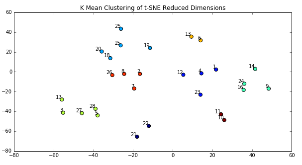
What is clear from the k-Means plot is that several songs are in clear clusters, such as songs 10 and 11, and 21 and 22. Song 10 is “Shakermaker” by Oasis, and song 11 is “All My Loving” by The Beatles. It makes sense that these songs are close together because both artists wrote similar styles of music. Not all Oasis’ songs or The Beatles’ songs are clustered together though. For example, “Yesterday” is closer in similarity to “Danse Macabre” by Camille Saint Saens than to other songs by The Beatles. That doesn’t make sense. The chart below maps song index to name for reference.
| audio_file_id | song | artist |
| 1 | Ain't No Grave | Johnny Cash |
| 2 | Danse Macabre | Camille Saint-Saens |
| 3 | Gimme Something Good | Ryan Adams |
| 4 | Mine | Taylor Swift |
| 5 | Symphony No.3 | Camille Saint-Saens |
| 6 | Roar | Katy Perry |
| 7 | Somewhat Damaged | Nine Inch Nails |
| 8 | Yesterday | The Beatles |
| 9 | Hurt | Johnny Cash |
| 10 | Shakermaker | Oasis |
| 11 | All My Loving | The Beatles |
| 12 | Back to December | Taylor Swift |
| 13 | Live Forever | Oasis |
| 14 | Wonderwall | Oasis |
| 15 | Don't Look Back in Anger | Oasis |
| 16 | Firework | Katy Perry |
| 17 | Little James | Oasis |
| 18 | Every Day is Exactly the Same | Nine Inch Nails |
| 19 | I Am the Walrus | The Beatles |
| 20 | Shake if Off | Taylor Swift |
| 21 | Bad Blood | Taylor Swift |
| 22 | Bad Blood | Ryan Adams |
| 23 | E.T. | Katy Perry |
| 24 | Every Reborn | Dario Marianelli |
| 25 | Supersonic | Oasis |
| 26 | I'd Like to Teachthe World to Sing | The New Seekers |
| 27 | The Swan | Camille Saint-Saens |
| 28 | Hurt | Nine Inch Nails |
While I was thinking of an explanation for why a Beatles song would be more closely related to a classical piece instead of other songs by The Beatles, I recalled two assumptions I was making that may not have been true. The first was that each song was autoencoded by itself. If the features that were learned were not in the same order, they would not align in the array that t-SNE was operating over. To correct this, the autoencoder would have to be trained on all of the songs together. The second assumption was that the music was accurately represented by the spectrogram. After all, the autoencoder was learning features and spatial relationships in the spectrograms rather than features about the raw audio data. As I mentioned before, the stereo to mono conversion and the loss of phase information in the creation of the spectrogram might cause vital information to be omitted from the network. Since it would take a lot more time to determine whether my second assumption was correct or not, I decided to test the first assumption and train the songs together.
Revised Deep Autoencoder
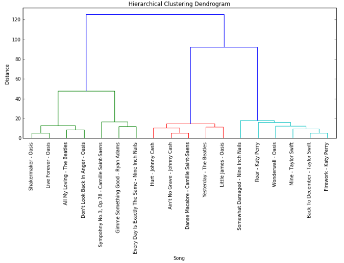
The second time around, I combined the audio files into a single matrix before passing them to the autoencoder. Due to system resource constraints, I had to chop off the last 10 songs and only train the autoencoder on 18 total songs. I used the same architecture and hyperparameters as the first model. The updated results are shown below for both the t-SNE and k-means visualizations. Notice that there are still distinct clusters appearing, but now the clusters make a lot more sense. Katy Perry and Taylor Swift songs are clustered together, suggesting that the autoencoder was able to learn something about the female voice, since the other songs are either classical or sung by males. Oasis and The Beatles are clustered together, which makes sense given the similarity in their musical styles. Songs with acoustic instruments are close together, which suggests that the autoencoder must be learning something about timbre or instrumentation as well. There were a couple exceptions, such as Oasis’ “Wonderwall” being more closely related to Taylor Swift than other songs by Oasis. Maybe the acoustic guitar in “Wonderwall” matched the acoustic sounds in Taylor Swift songs better. Whatever the case, the autoencoder is clearly learning distinct features and recognizing similar sounding songs accurately.
Below is an agglomerative hierarchical clustering dendrogram that more clearly displays the results of the autoencoder and t-SNE algorithms.
For curiosity’s sake, I plotted the encoded image for one of the songs below. Each encoded image is a dimension reduced representation of the original spectrogram, just like this:
The above image of an encoded song is expanded out to the original input dimensions in the decoder piece of the autoencoder. The expansion was accomplished through the use of upsampling and convolutional layers. The result of the reproduction is below, and the original spectrogram for the same song is below that.
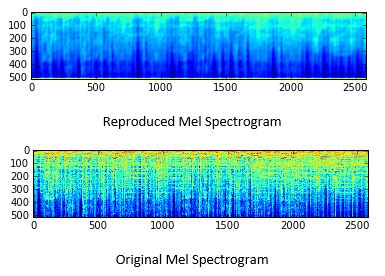
It is clear to see that even though the reproduction looks like a shadow of the original, there are structural similarities. I’m confident that with a deeper network, or by making any of the improvements I’m about to describe, the reproduction could become even more accurate, and the resulting clusters could be even more insightful.
Ideas for Future Improvements
While convolutional networks are great for learning spatial structure, recurrent networks are useful for time sequences. I wanted to add a long-short term memory (LSTM) layer at the beginning of the encoder piece to learn repeating sequences in the music, but I could not, because I had no reliable way to determine which time steps to use. Since music is written in bars, my thoughts were that the ideal time step would be the time signature of the song. So if a song had 4 beats per measure, then the time step could be 4. However, there is currently no way to determine the time signature of an audio file. The best option might be to tune the time steps parameter until the results had the lowest error or validation loss, but regardless of what it tuned to, the resulting time step would be some combination of the time signatures of all the songs in the dataset. If some songs were 4:4 time, and others 5:8, then the tuned time step would match neither. An ideal model would use a time step parameter that could adapt to whatever sample was being trained, though doing that would require knowing the precise time signature for each song.
If I were to expand the autoencoder, I would focus on adding the LSTM layer. Doing this with Keras would require reshaping the input layer to a long sequence, essentially stacking the columns together, assuming the columns of the input image represent points in time. Other improvements could be made by adding more layers, or by expanding the layers that already exist. I did not try either in this experiment because I had already run out of RAM training on 18 samples with the existing architecture. A more powerful computer could undoubtedly handle more layers, which would likely improve the model’s accuracy.
Another improvement that is possible would be to enrich the data by adding the second channel for each wav, after the conversion to mono. There would then be 2 samples per song. Rather than mathematically combining the channels into 1 input, each could be trained separately in identical autoencoders, and then combined in an ensemble model. This would be similar to how human hearing works. Each ear receives separate input and the brain combines them in a way that makes sense to us.
Several more improvements could be made by adding features related to the metadata of the songs, like artist, album, or year, or by adding features like the ones I originally calculated. The deep convolutional autoencoder could even be combined with traditional collaborative filtering systems. The recommendations would then be a blend of user input and raw audio signal.
These are just a few of many ways to improve the model, but this experiment has shown great potential for music recommendation with deep learning.